

Data from the 2026 market cycle reveals a structural transformation in decentralized finance liquidity provision. The era of triple-digit annual percentage yields has concluded, replaced by a yield environment where risk-adjusted returns determine protocol viability. This analysis examines the mechanisms driving APY compression, quantifies impermanent loss under varying market conditions, and establishes a framework for differentiating sustainable from unsustainable yields.
The 2026 Yield Environment: A New Baseline
The current DeFi market exhibits yield compression across all major protocols. Stablecoin lending on platforms like Aave and Compound generates 3% to 12% APY, while ETH staking yields stabilize at 3.0% to 3.8%. DEX liquidity pools show variable returns ranging from 2% to 8%, dependent on trading volume and pool composition.
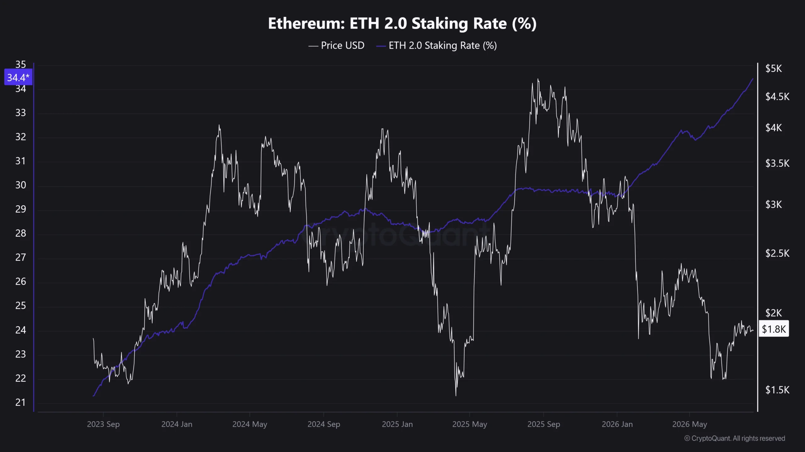
This compression represents a departure from the 2021 cycle, where protocols advertised APYs exceeding 50% and, in some cases, quadruple-digit returns. The transition reflects reduced token emission schedules, lower leverage demand, and diminished speculative trading activity.
Total stablecoin supply reached $312 billion in 2026, indicating capital deployment rather than capital exit. However, this capital gravitates toward yield-bearing stablecoin products such as sUSDS and SyrupUSDC, which offer predictable returns with lower principal risk.
Bull Market APY
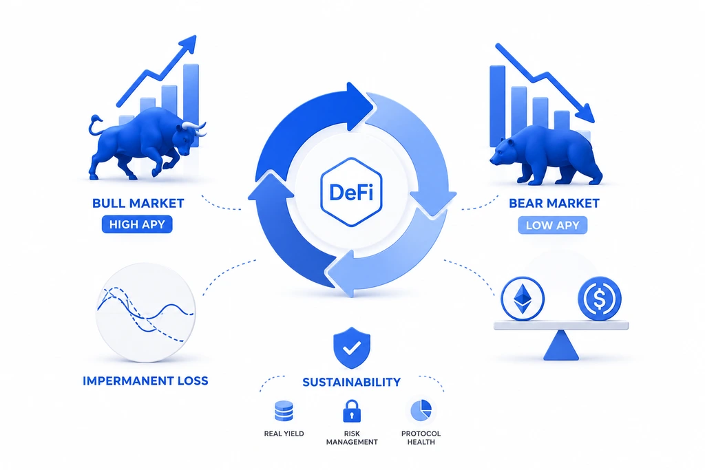
Bull market APY escalation originates from three primary mechanisms: transaction volume multiplication, leverage demand amplification, and protocol incentive competition.
Rising asset prices generate higher DEX trading volumes, increasing fee revenue for liquidity providers. Simultaneously, traders seeking leveraged long positions drive borrowing rates upward on money markets. Protocols respond with emissions-based liquidity incentives, creating an additional yield layer that compounds the nominal APY displayed to users.
Impermanent loss manifests asymmetrically during bull phases. A liquidity provider depositing ETH-USDC observes the AMM algorithm systematically selling their ETH position as prices appreciate. A 2x price change generates approximately 5.7% impermanent loss before accounting for fee generation. At 5x price appreciation, the loss exceeds 20%.
The late-cycle entrant faces the highest risk concentration. These providers accept full price exposure and IL costs while receiving diluted reward tokens. APY optimizers frequently rotate into pools at peak APY levels, precisely when the risk-reward ratio reaches its least favorable configuration.
Bear Market APY
Bear market yield behavior demonstrates compression across all asset classes except stablecoin-based products. Trading volume contraction reduces fee generation. Leverage demand declines as traders deleverage positions. Protocol emission schedules face downward pressure as treasury management becomes prioritized over growth expenditure.
Capital rotation characterizes bear market behavior. Liquidity migrates from volatile asset pools to stablecoin pairs, seeking preservation of principal above yield maximization. This rotation explains the increased TVL observed in stablecoin lending protocols despite declining total DeFi TVL across the industry.
Impermanent loss mechanics invert during bear markets. A liquidity provider holding a volatile asset paired with a stablecoin experiences the AMM algorithm accumulating more of the declining asset. The position increasingly represents the depreciating token, compounding losses through both price action and pool rebalancing.
Protocols demonstrating stable APY during bear phases establish credibility with institutional capital providers. A sustainable 8.5% stablecoin yield during market contraction carries greater value than a 20% volatile asset yield, as the latter reflects uncompensated risk exposure.
Impermanent Loss: A Mathematical Quantification
Impermanent loss expresses the difference between a liquidity position’s value and the value of simply holding the underlying assets. The loss calculation depends exclusively on price ratio change, independent of absolute price movement magnitude.
The standard IL formula for a 50/50 pool:
IL = 2√r / (1 + r) – 1, where r represents the price ratio at withdrawal versus deposit.
This formula yields quantifiable loss thresholds:
High volatility regimes amplify IL beyond fee generation capacity. A pool generating 10% annual fees faces IL erosion exceeding 15% during a 3x price movement, producing a net negative return despite positive fee accumulation.
IL converts from impermanent to permanent when the price ratio fails to return to the deposit level. This condition describes the majority of market cycles, as asset prices rarely revert precisely to historical entry points.
Sustainable Versus Unsustainable Yields
Yield sources divide into organic revenue and incentive-based emissions.
Organic yield components include DEX transaction fees, lending interest payments, arbitrage profits, and liquidation penalties. These revenue streams derive from genuine economic activity and persist independent of protocol tokenomics.
Incentive-based yield components include protocol token emissions, liquidity mining rewards, initial liquidity bootstrapping incentives, and bribe/vote markets. These represent value transfers from protocol treasuries to liquidity providers, subsidized by future token dilution.
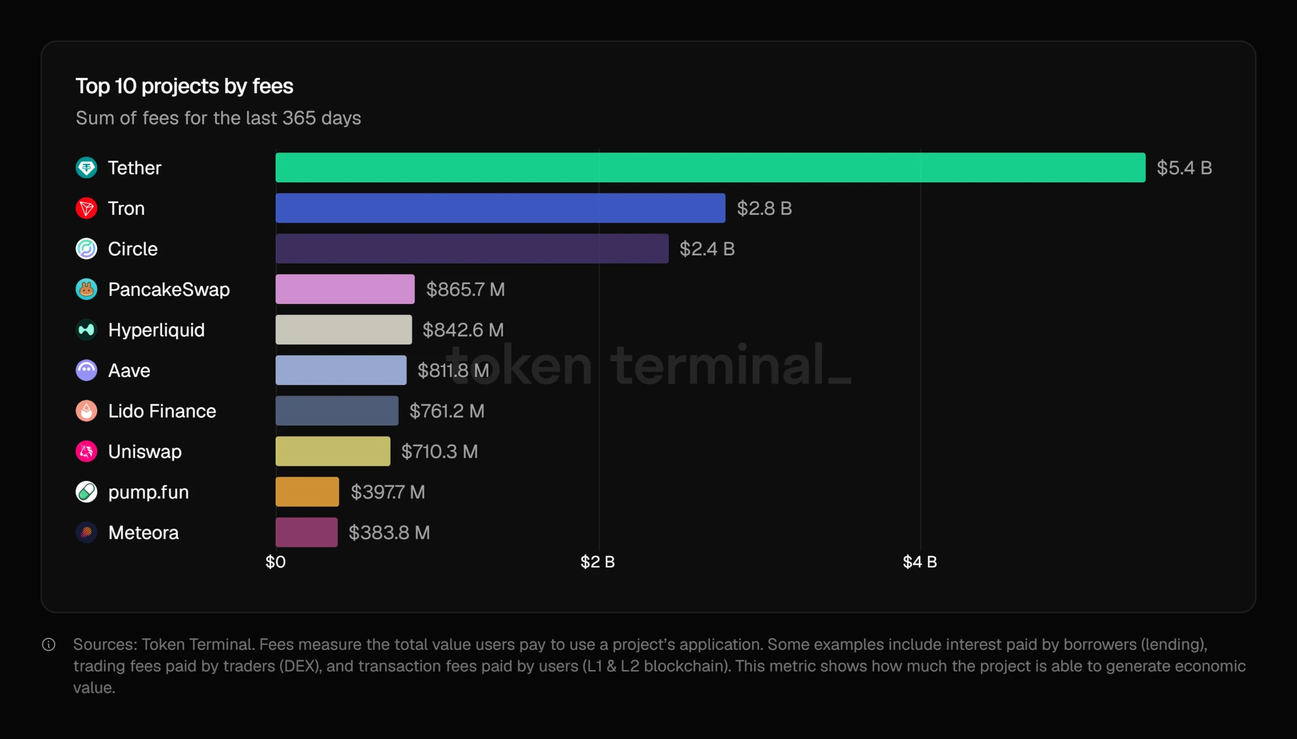
The sustainability threshold calculation compares protocol revenue against reward expenditures. Protocols distributing rewards exceeding their revenue demonstrate negative gross profit margins, indicating reliance on token inflation rather than economic activity.
Current DeFi benchmarks show most protocols operating at reward-to-revenue ratios exceeding 2:1. This indicates that for every dollar of organic revenue, protocols distribute two dollars in token emissions. This ratio proves unsustainable over extended periods, forcing eventual emission reductions.
The Yield Decomposition Equation
The net yield calculation incorporates costs and risks often excluded from advertised APY figures:
Net Yield = Gross APY – IL – Protocol Fees – Execution Costs – Risk Premium
Execution costs include swap slippage, rebalancing gas expenditure, and withdrawal penalties. A 100% gross APY pool with 20% IL exposure, 5% fees, and 10% execution costs produces a net yield of 65% before considering counterparty and smart contract risks.
Risk-adjusted yield further adjusts for volatility, protocol security, and regulatory exposure. A 50% APY on a high-risk protocol may underperform a 10% APY on an established platform when factoring these adjustments.
Implications for Liquidity Provision
Liquidity providers operating in the 2026 environment must implement yield analysis beyond headline APY figures.
The principal consideration involves assessing the proportion of organic versus incentive-based yield. Protocols deriving over 50% of APY from emissions face future yield compression risk as emission schedules decline.
Impermanent loss mitigation requires selecting correlated asset pairs with lower price ratio variance. Stablecoin-stablecoin pools minimize IL but generate lower fees. Volatile-stablecoin pools offer higher fee potential with increased IL exposure.
Position management timing influences returns. Providers entering during low volatility periods and exiting during low volatility periods minimize IL. Entering during volatility extremes, regardless of price direction, increases negative return probability.
The Real Yield Standard
The industry demonstrates convergence toward real yield metrics as institutional capital demands transparency. Real yield subtracts token emissions from gross APY, revealing the return generated by economic activity.
Protocols achieving positive real yield maintain viability across market cycles. These protocols demonstrate product-market fit through fee revenue, independent of token appreciation or emission programs.
The real yield benchmark for DeFi protocols in 2026 falls between 2% and 6%. Returns exceeding this range require scrutiny of emission components and risk exposures.
The Rationalization of DeFi Yields
The DeFi yield environment has undergone structural rationalization since the 2021 cycle. Nominal APY inflation through token emissions has given way to capital preservation strategies and risk-adjusted return optimization.
Market participants no longer evaluate protocols solely on headline yields. The sophisticated liquidity provider analyzes yield composition, IL exposure, execution costs, and protocol revenue sustainability before deployment.
The sustainable yield ceiling for DeFi in 2026 approximates 4% to 8% for stablecoin positions and 2% to 6% for volatile asset positions, adjusted for market conditions.
DeFi protocols maintaining APY above these ranges attract liquidity but should expect emission compression and consequent APY reduction over the following quarters. The rational market allocates capital to protocols demonstrating revenue sustainability rather than temporary incentive programs.
This rationalization phase, while reducing visible APYs, establishes the foundation for institutional capital deployment and long-term DeFi market growth.

Isai Alexei is a journalist and financial analyst covering cryptocurrency markets and traditional securities for Blockchaindose. He has spent ten years analyzing digital assets, trading activity, and market structure.